
JPOSNA® Special Edition
Advances in Pediatric Orthopaedic Education and Technical Training
PLIRSP: Planning for Limb Reconstruction Using Slide Presentation Software
Universidad de los Andes, Santiago, Chile
Correspondence: Alejandro K. Baar, MD, Department of Orthopedic Surgery, Clinica Universidad de los Andes, Av. Plaza 2501 – Las Condes, Santiago de Chile. E-mail: [email protected]
Received: April 17, 2022; Accepted: April 18, 2022; Published: August 15, 2022
DOI: 10.55275/JPOSNA-2022-0066
Volume 4, Number S1, August 2022
Introduction
Before the era of digital radiology, we had to deal with “old plain films.” Those pictures did not have the resolution that the new generation of x-ray machines generate today. Moreover, having a “physical” film forced the surgeon to use school tools, like pencils, protractors, and erasers to measure and analyze deformities. In those days, planning a deformity correction used to be a hard task. After lines and angles were measured on the x-ray films, you had to trace them over a paper sheet; then, with the help of scissors, the proposed osteotomy was recreated and the segments were realigned. It is interesting to see on page 22 of Paley’s Principles of Deformity Correction, how Paley himself is measuring long-leg films.1
Digital technology creates x-rays with less radiation, better resolution, and extraordinarily easy storing and sharing capabilities. This is what we know as a Picture Archiving and Communication System (PACS). Digital Imaging and Communications in Medicine (DICOM) is a worldwide standard for the storage and transmission of medical imaging. The standard, therefore, defines both a file format and a networking protocol. Multitude DICOM viewers are available—some freeware, some paid, some targeted at medical students or seasoned experts and each with different specifications, systems requirements, add-ons, and capabilities. Most of them give access to several tools for image analysis. It is possible to measure length, angles, and diameters directly on the screen. However, when planning is required, it is necessary to have access to CAD (Computerized-Aided Design) software. This type of software provides tools like copying, pasting, cropping, angulation, translation, etc., and offers a wide selection of implant templates, which help make limb deformity planning fast and easy. However, these software tools can be complex, and training is usually needed before mastering them. Furthermore, these software tools can be expensive, and often a renewable subscription is mandatory.
An extraordinary educational tool, to be used with tablets (either iOS or Android), was released in 2012 by Drs. Shawn Standard and John Herzenberg, from the International Center for Limb Lengthening, Baltimore, MD. The Bone Ninja app has made deformity correction planning ridiculously simple.2 Since its introduction, it has replaced the pencil and goniometer during the yearly Baltimore Limb Deformity Course and has become a “favorite” among limb reconstruction surgeons “who own a tablet.” I use quotes because, unfortunately, many surgeons do not have one.
For those who do not have access to a tablet but need to plan limb reconstruction, I propose a simple method using slide presentation software (SPS), such as Microsoft’s PowerPoint or Apple’s Keynote. I call it PLIRPS, which stands for Planning for Limb Reconstruction Using a Slide Presentation Software.
I have been using this method since 2008, after completing a fellowship in limb lengthening and reconstruction, when digital x-rays were already available but the Bone Ninja app was not.
This method can be used to teach residents and fellows how to plan a deformity correction. It allows them to practice different alternatives for bone correction and implant selection and then save this information so that it can be used during surgery to guide the correction.
Description of Simulation Exercise
The surgeon needs access to SPS, such as PowerPoint or Keynote. Both work well, but Keynote has one special trick that allows crop and rotate.
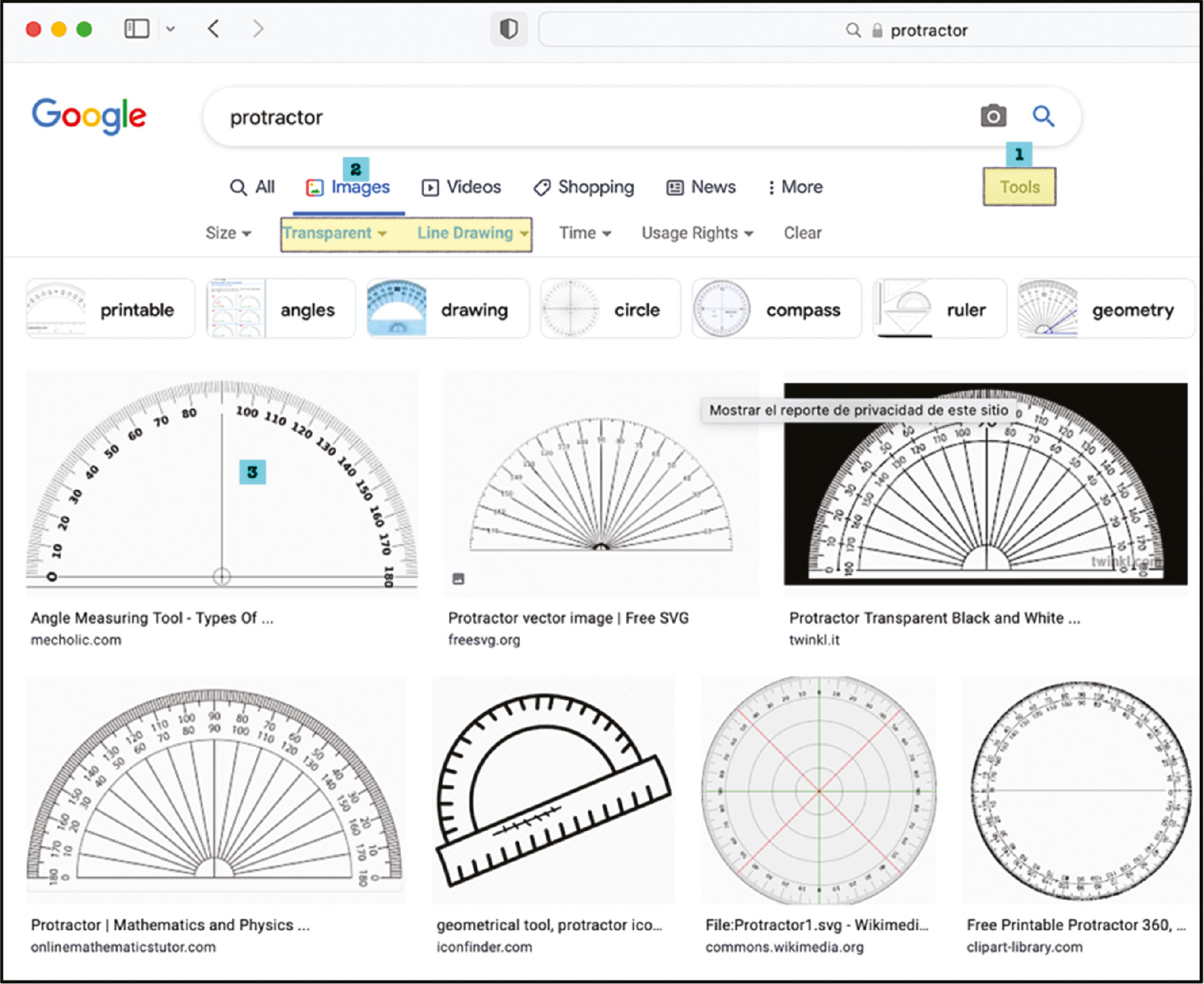
Google the words “protractor” and “ruler” and download the images. Try to find one with a transparent background. They are usually in .png format (Figure 1).
Figure 1. In your favorite internet browser, look for a protractor. 1) Go to the tools tab, 2) In the images tab, select transparent color and line drawing, 3) Choose your favorite protractor, and save it as a .jpg or .png image.
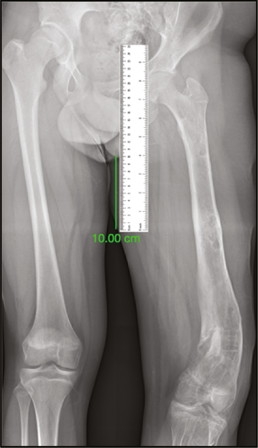
The patient’s x-rays need to be saved in .jpg or .png format in order to export them from your SPS. The images will need to include a scale marker so that measurements can be made directly on the radiograph. If your facility does not obtain x-rays with magnification markers on the images, you can create your own scale marker. This can be done by drawing a 10 cm line on the image in a place where it will not interfere with your planning.
Open your SPS, and import the images of the x-rays, the transparent protractor, and the ruler. Use your scale marker line to calibrate the ruler. It means you need to resize the ruler till the 10 cm mark matches your marker line (Figure 2).
Figure 2. The scale marker is displayed on the x-ray image. A 10 cm line was drawn away from the deformity to be corrected. This is done with any DICOM viewer. Save the image, with the marker included, as a .jpg or .png file. Search the internet for a ruler; again, save the image. Open your preferred SPS and import the x-ray image and the ruler. Let the 10 cm line correspond to the 10 cm mark on the ruler.
When using traditional black background x-rays, use a black background on your slides. If you are working with “negative x-rays,” use a white background.
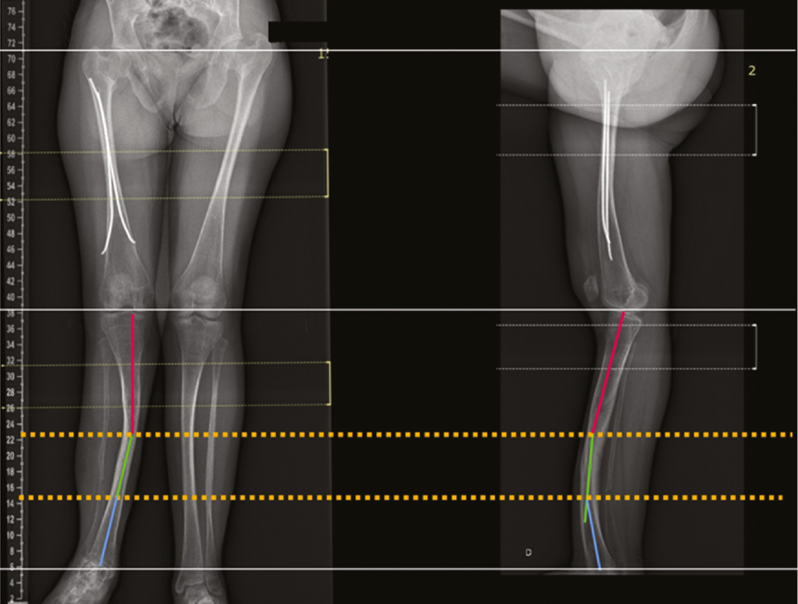
Try to accommodate AP and LAT views together in the same slide, taking care to level femoral heads, femoral condyles, tibial plateau, and tibial plafond. For this, you can use the figure tool, select a line, and set it horizontally. Move and resize the x-rays in a way that the most proximal horizontal line is touching the same reference point on both AP and LAT views. Add another horizontal line distally, again, touching the same reference point on both x-ray projections. Remember to add a scale marker on each x-ray (Figure 3).
Figure 3. AP and LAT views are put together in a slide. The long, thin, and white horizontal lines are used to match the same anatomic landmark on both projections. Here, one is over the top of the femoral head, the middle one is at the knee joint line, and the distal one is at the tibial plafond. The yellow dotted lines represent the level of deformity apex. In this example, there is one proximal apex seen at the same level on both projections, which means an oblique plane deformity. There is an additional apex at the distal tibia, seen just on the LAT projection.
If you are familiar with the malalignment test (MAT),3,4 the next steps are straightforward: Draw mechanical and/or anatomical lines in the corresponding segments using different colors for proximal and distal segments. Align the protractor with these lines, measuring the different angles (LDFA, MPTA, etc.) You also will find the CORA (center of rotational angulation) or apex where the lines cross each other5,6 (Figure 4).
Figure 4. AP and LAT views of a severe deformity of the leg. Proximal and distal mechanical axes were drawn, and the apex corresponds to the crossing point. Now, the protractor image is imported. Its base must be aligned with any of these axes. Read the angles and write them using a text box.

Now, it is time to plan the osteotomy and simulate the correction. For this step, you will need to copy and paste each x-ray a couple of times.
As you already found the apex, and you know where you are going to do the osteotomy, you can crop each copy of the x-ray in a way you get two segments—one proximal and one distal to the planned osteotomy. To make it very schematic, I also suggest to copy and paste the axis lines of each segment. At this point, it is very useful to pick the bone segment with its corresponding lines together, right-click on your mouse, and group them. Each segment, with its axis lines, will move as a one-piece block.
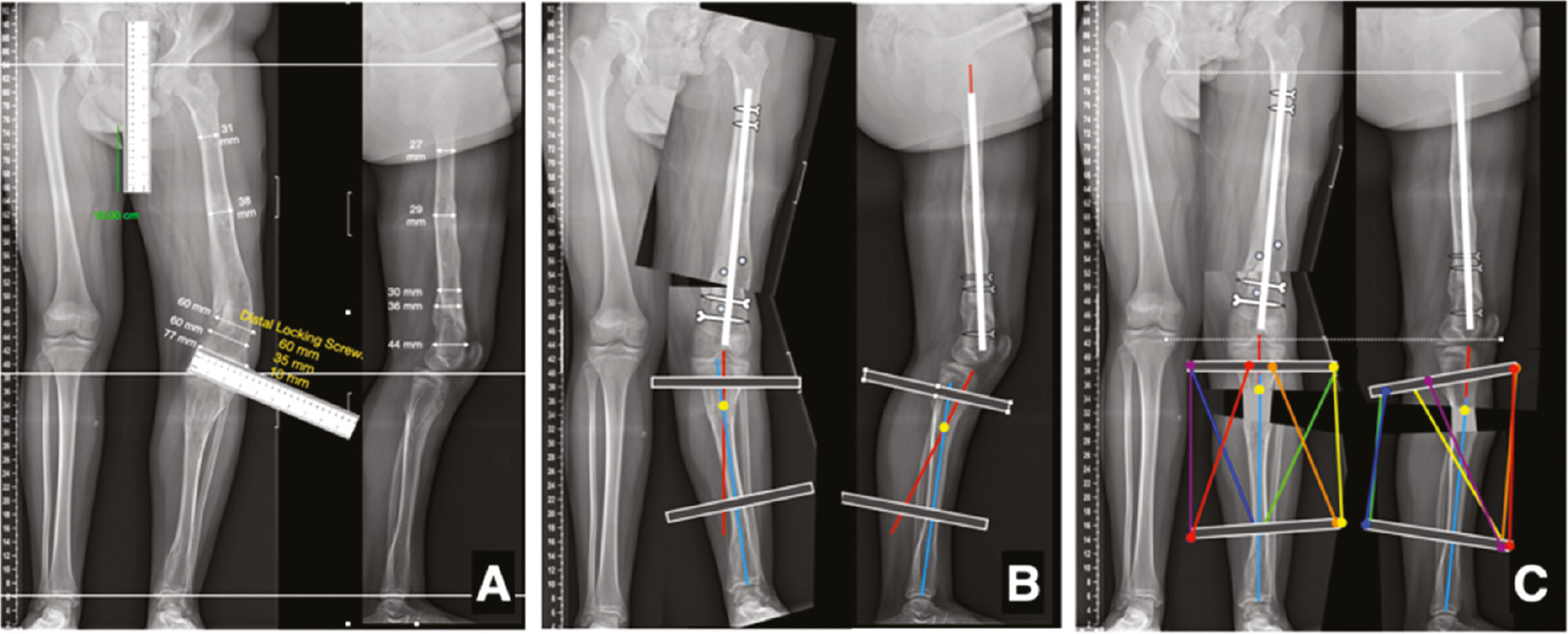
Finally, taking into account the angles you previously measured, you can take one of the segments and rotate it using the rotation tool until the desired correction is achieved (Figure 5). Moreover, you can use your calibrated ruler to measure the size of the opening or closing wedge that you are going to use.
Figure 5. The steps needed for deformity correction planning are depicted. A) Draw the axis lines on each segment, including joint orientation lines. Use the protractor to measure anatomical and/or mechanical articular angles. Find the apex and measure its magnitude. B) Copy and paste the x-ray image and then crop it, keeping just the side you want to work with. C) As two apexes were identified, three copies are done, and each one is cropped to recreate the segment to be corrected. D) In this exam, the distal segment is rotated 10 degrees and the middle segment 16 degrees, according to previous measurements. In PowerPoint, the image can be directly rotated, scrolling any corner of the image with the mouse. As the rotation occurs around the center of the image, a lot of translation is expected, so you will need to move the segment with the keyboard arrows or using the mouse. E) Finally, select all the bone segments and their axis, and group the images together (right button and select group). Rotate the full image as a unit until it is in an anatomic position.

Be aware that the image rotation occurs around the center of the image (not necessarily the CORA). This creates a translation deformity, so you will need to move the segment with the keyboard arrows or using the mouse.7
If you are using Keynote, there is a tool to facilitate the angular correction and also make your presentation more aesthetic. Keynote allows you to crop a rotated image. This feature avoids the patchwork appearance of corrected images (Figure 6).
Figure 6. Keynote special feature: rotation of the cropping frame. A) The bone segment to be corrected was previously defined during deformity analysis. Select the moving segment (distal in this case) and use the crop function. Go to the rotation tool (highlighted in green). B) Rotate the cropping frame until its sides are parallel to the long axis of the segment, (and/or bottom and top lines are parallel to joint lines). In this case, 23 degrees of rotation was necessary. C) Complete the cropping by either pressing the mouse button or the enter tab on the keyboard. The distal segment will still be deformed. Now pick this segment again (without cropping!) and rotate back to the original angle—in this case, 23 degrees. This will automatically make the correction. D) Finally, crop the corrected segment to align its margins with the proximal segment.

Once you select the segment that you would like to rotate and crop, select the “crop” function. Then, using the rotation tool, align the top edge of the frame so that it is parallel to the joint line of your segment. After pressing enter, select the picture again without the crop tool and rotate it back to its original position. You will get a nice image with its frame aligned.
Bonus track: Each implant system has its own brochure with specifications. (For instance, a nailing system will present the different lengths and diameters, or a plating system will tell you the sizes, number of holes, and interspacing between them.) Download an image of your preferred implant, calibrate it with the ruler, and try it on the corrected bone. You can also draw your own implants, taking into account the dimension you have learned from the brochures (Figure 7).
Figure 7. Using the ruler, the length and diameter of the chosen implant can be obtained. The image of a Meta-Nail (Smith and Nephew Inc., Memphis, TN) was taken from the surgical technique brochure and added to the x-rays to simulate the fixation and planning the position of blocking screws and external fixator pins.

Finally, you can also draw an external fixator, even a hexapod, but this will take time and it is just for fun (Figure 8).
Figure 8. A) AP and LAT x-rays of a patient with Ollier’s disease and a varus deformity of the left distal tibia as well as recurvatum and shortening of the left tibia. Level lines on both projections. The 10 cm scale line and the ruler are depicted. Note that even the length of each locking and blocking screws can be known in advance. B) Simulation of femoral correction with an intramedullary rod. Little dots represent blocking screws to be used. Axis lines are drawn in the tibia and external fixation rings are added. The diameter of these rings can be measured with the ruler. C) Final correction, including both femur and tibia. Color lines represent hexapod struts. After the tibial correction was done, both proximal and distal tibia segment along with the rings and strut are grouped. As a single piece, the tibia is extended under the femur (knee extension) to simulate the final position.
Summary
Deformity correction requires careful planning. In “ancient times” it was done with a pencil, protractor, and paper dolls. The arrival of digital technology has made x-ray analysis much easier. However, most PACS viewers allow measuring angles and distances. For further planning, it is necessary to have CAD software, which needs special training and is expensive. The Bone Ninja app is suitable for tablets, has mind-blowing features, is very easy to learn, but requires access to a tablet. As an alternative, I propose a cheap, simple, fun, and accurate method for planning using SPS, which is widely available. The plans can be easily saved, sent by email, or even printed to be used for reference in the OR, even if a computer is not available.
Disclaimer
The author serves as a speaker and paid consultant for OrthoPediatrics and Orthofix.
References
- Paley D. Principles of Deformity Correction. 1st Edition, Springer-Verlag Berlin Heidelberg 2002. ISBN 978-3-642-63953-1. DOI: 10.1007/978-3-642-59373-4.
- Standard SC, Herzenberg JE, Conway JD et al. The Art of limb alignment. 3rd Edition. Rubin Institute for Advanced Orthopedics, Sinai Hospital of Baltimore; 2014.
- Paley D, Tetsworth K. Mechanical axis deviation of the lower limbs. Preoperative planning of uniapical angular deformities of the tibia or femur. Clin Orthop Relat Res. 1992;(280):48–64.
- Paley D, Tetsworth K. Mechanical axis deviation of the lower limbs. Preoperative planning of multiapical frontal plane angular and bowing deformities of the femur and tibia. Clin Orthop Relat Res. 1992;(280):65-71.
- Paley D, Herzenberg JE, Tetsworth K, et al. Deformity planning for frontal and sagittal plane corrective osteotomies. Orthop Clin North Am. 1994;25(3):425–465.
- Paley D, Pfeil J. Prinzipien der kniegelenknahen Deformitätenkorrektur [Principles of deformity correction around the knee]. Orthopade. 2000;29(1):18-38. German.
- Paley D. Correction of limb deformities in the 21st century. J Pediatr Orthop. 2000;20(3):279-281.